
Walmart Sales Insights: A Predictive Modelling Approach
In this project, my objective was to accurately predict weekly sales using time-series models and understand the drawbacks of traditional ML models and deep learning models with respect to the features of this dataset. The project’s code and detailed methodology are accessible here.
What Drives the Sales of the World’s Largest Retailer?
As of November 2023, Walmart is the world’s largest retailer, with global sales of over $600 billion, and operates on a scale that generates immense volumes of data. This project delved into analyzing this data to decode performance trends and identify its approach to financial and operational efficiency. The aim was to understand the impact of factors like store size, holidays, and economic indicators that affect sales, and how these insights could be used for accurate revenue predictions, effective marketing campaigns, efficient inventory management, and the ability to anticipate and meet seasonal demands.
Some insights from the Exploratory Data Analysis
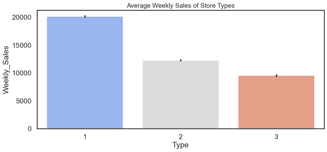
- The popular type of store is Type A - Walmart Supercenter, with the highest average weekly sales.
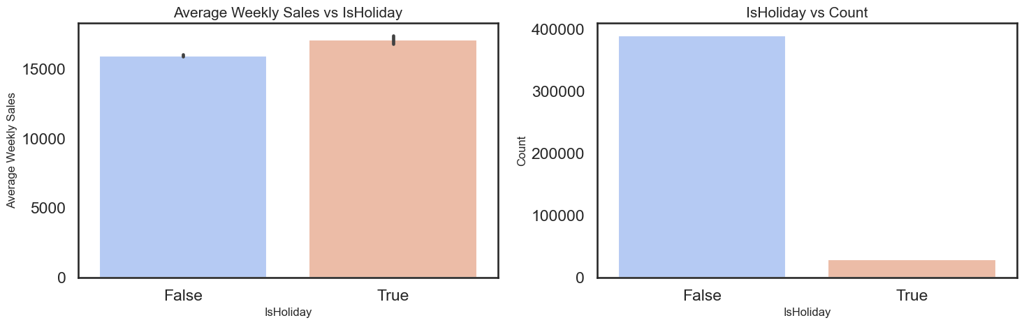
- Holiday weeks, specifically weeks 5, 35, 46, and 51, demonstrate a significant spike in sales, as indicated by the higher average sales per week compared to non-holiday periods. Despite accounting for a smaller portion of the data, these weeks markedly impact overall sales figures.
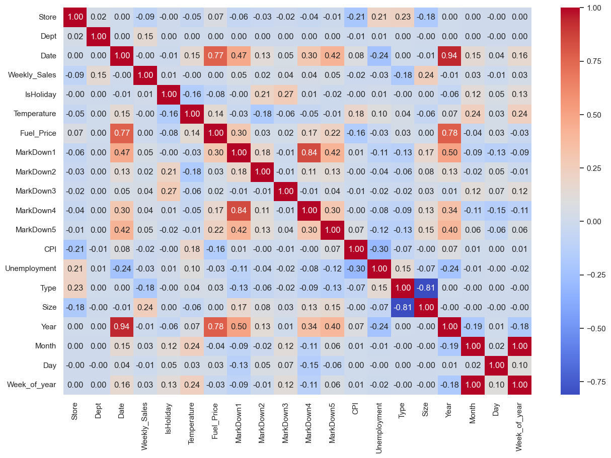
- The variables Temperature, Fuel Price, Consumer Price Index (CPI), and Unemployment exhibit a very low correlation with weekly sales, suggesting their limited impact on sales forecasting.
Additionally, the ‘month’ and ‘day’ columns, showing a high correlation with the ‘week’ data, are redundant and can be dropped.
Furthermore, Markdowns 4 and 5 are found to be highly correlated with Markdown 1, indicating an overlap in information, and thus, they can be streamlined by removing them from the dataset.
Model Implementation Details and Modifications
- Model Selection: The SARIMA model was selected due to the dataset’s characteristics, particularly the annual seasonal component. This model is an extension of the ARIMA model, specifically designed to handle seasonality.
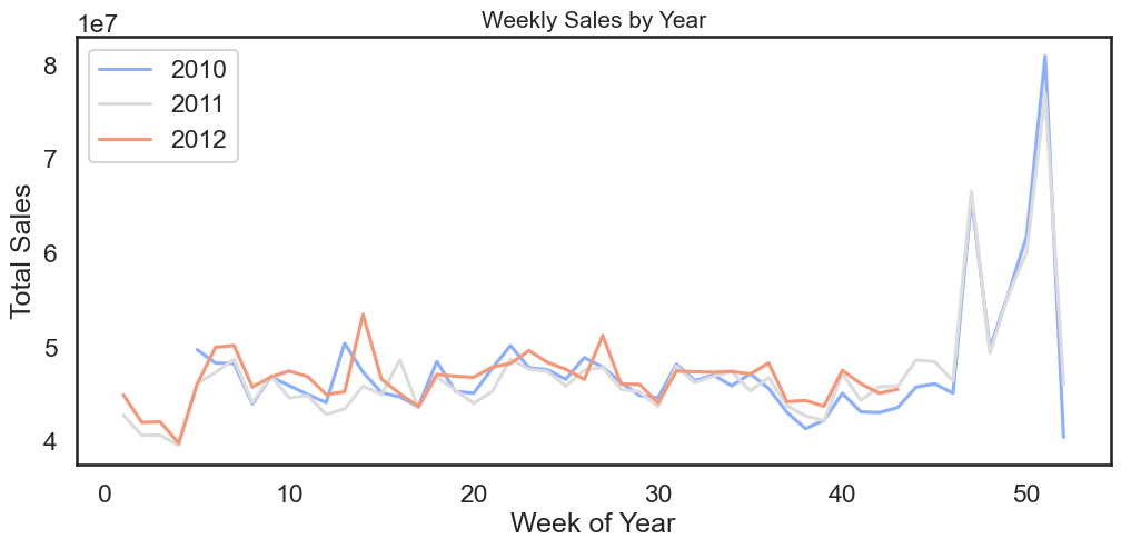
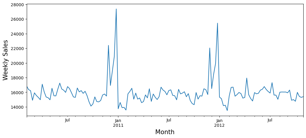 We can see the seasonality in the weekly sales data, which clearly tells its a time series problem.
Parameter Determination: The SARIMA model’s implementation involved specifying three major hyperparameters for autoregression (AR), differencing (I), and moving average (MA) for both seasonal and non-seasonal components, along with an additional parameter for the period of the seasonality. The parameters included:
p and seasonal P (number of AR terms)
d and seasonal D (differencing required)
q and seasonal Q (number of MA terms)
Lag (seasonal length in the data).Parameter Estimation Process: To estimate these parameters, the Auto-Correlation Function (ACF) and Partial Auto-Correlation Function (PACF) graphs were plotted for a rough estimation of the parameters. This was followed by a grid search to find the best combination of values based on the Akaike Information Criterion (AIC) scores.
Model Fitting: The final SARIMA model was fitted using the parameters (3, 0, 4) for the non-seasonal component and (1, 1, 1, 52) for the seasonal component. This configuration was determined to have the least AIC value, indicating optimal model performance. The model was then used to calculate the Weighted Mean Average Error (WMAE) for evaluation. The WMAE was found to be 438.62 and the predictions are as shown below.
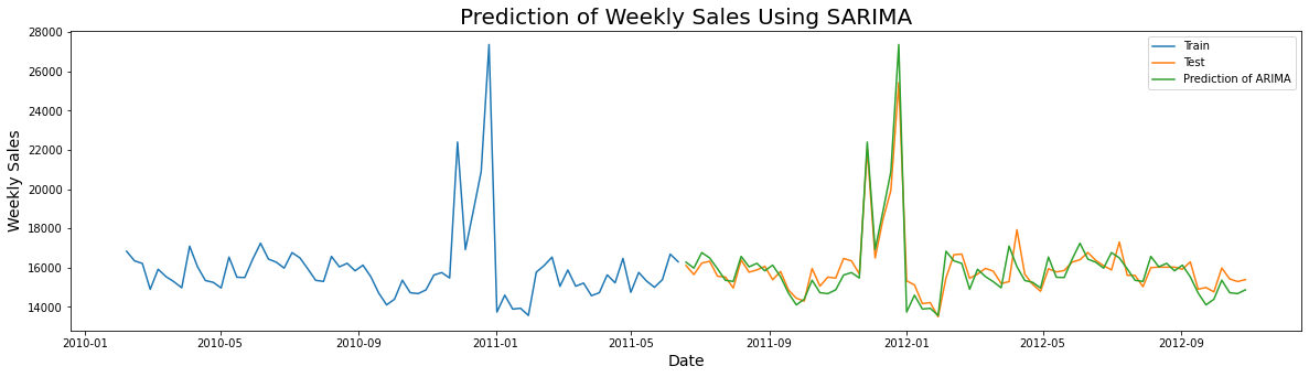
- Comparison with Other Models: In addition to SARIMA, several other models were tested and their limitations are as follows:
- Traditional ML Models- Regression models like Ridge Regressor, Random Forest, and XGBoost provided good WMAE scores but struggled with extrapolation, i.e., making predictions outside the known data range, leading to high errors.
- Deep Learning Models- Deep learning models such as LSTM and MLP faced challenges due to their high memory bandwidth and computational demand. These models require large hidden layers and deeper networks, which can be resource-intensive and inefficient for many systems, particularly when dealing with the linear layers present in each cell of the network.
- Conclusion: The SARIMA model provided the most accurate sales predictions due to:
- Autoregressive Nature of Data- The dataset exhibited a strong autoregressive pattern, meaning the weekly sales at any given time were highly dependent on the sales in previous weeks. Autoregressive models like SARIMA are particularly adept at capturing and modeling this kind of data pattern.
- Handling of Seasonality- SARIMA, being specifically designed for time series data with seasonality, was able to effectively capture and predict the cyclic patterns observed in the sales data over a three-year period. This capability to detect and utilize seasonality in the data was a significant factor in its superior performance.