Statistical A/B Testing

A/B Testing

A/B testing stands as a paramount methodology in the realm of controlled experiments, particularly in enhancing web marketing initiatives. This technique empowers decision-makers to select the most effective website design by analyzing the performance metrics of two distinct alternatives, labeled as A and B.

A/B testing involves presenting two variant designs, A and B, to website visitors in a random manner. Subsequent to their interaction, data regarding their engagement is amassed through web analytics tools. This data serves as a foundation for applying statistical tests to ascertain if there exists a significant difference in performance between the two designs.

The assessment of a website’s performance can be quantified using diverse metrics. Discrete or binomial metrics, which only assume the values 0 and 1, include:

• Click-through rate: The likelihood of a user clicking on an advertisement.
• Conversion rate: The probability of a user, upon seeing an advertisement, becoming a customer.
• Bounce rate: The chance of a user navigating to a different page within the same website after their initial visit.

Conversely, continuous or non-binomial metrics afford a range of values beyond binary outcomes. Notable examples of continuous metrics encompass:

• Average revenue per user: The monthly revenue contribution per user.
• Average session duration: The typical length of a user’s visit on the website.
• Average order value: The average total value of a user’s order.

Statistical Significance

To discern the relative success of designs A and B, merely comparing average values falls short of capturing the statistical significance of observed differences. It’s crucial to evaluate the probability that these differences could have occurred by chance.

This evaluation involves conducting a two-sample hypothesis test. The null hypothesis (H0) posits that designs A and B are equally effective, gauged by metrics such as click-through rate or average revenue per user. The level of statistical significance is determined by the p-value, representing the likelihood of encountering a discrepancy between our samples as substantial as or more than our actual observation.

Selecting the appropriate alternative hypothesis (Ha) necessitates deciding between one-tailed and two-tailed tests. Given the absence of preliminary bias towards either design, a two-tailed test is recommended. This approach assumes Ha to embody the proposition that designs A and B differ in effectiveness.

The computation of the p-value, indicative of the probability of observing such disparities by chance, is contingent upon the underlying data distribution. We will explore how to calculate this for both discrete and continuous metrics.

Discrete Metrics

Let’s first consider a discrete metric such as the click-though rate. We randomly show visitors one of two possible designs of an advertisement, and we keep track of how many of them click on it.

Let’s say that from we collected the following information.

nX = 15 visitors saw the advertisement A, and 7 of them clicked on it. nY = 19 visitors saw the advertisement B, and 15 of them clicked on it.

At a first glance, it looks like version B was more effective, but how statistically significant is this discrepancy?

Fisher’s exact test

Using the 2x2 contingency table shown above we can use Fisher’s exact test to compute an exact p-value and test our hypothesis.

To understand how this test works, let us start by noticing that if we fix the margins of the tables (i.e. the four sums of each row and column), then only few different outcomes are possible.

The key observation is that, under the null hypothesis H0 that A and B have same efficacy, the probability of observing any of these possible outcomes is given by the hypergeometric distribution.

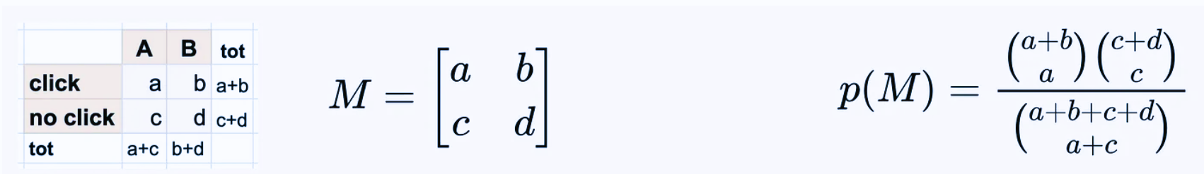
Using the above formula we obtain:

• the probability of seeing our actual observations is ~4.5%
• the probability of seeing even more unlikely observations in favor if B is ~1.0% (left tail)
• the probability of seeing observations even more unlikely observations in favor if A is ~2.0% (right tail)

Fisher’s exact test gives p-value ≈ 7.5%.

Pearson’s chi-squared test

Fisher’s exact test has the important advantage of computing exact p-values. But if we have a large sample size, it may be computationally inefficient. In this case, we can use Pearson’s chi-squared test to compute an approximate p-value.

Call Oij the observed value of the contingency table at row i and column j. Under the null hypothesis of independence of rows and columns, i.e. assuming that A and B have same efficacy, we can easily compute corresponding expected values Eij. Moreover, if the observations are normally distributed, then the χ2 statistic follows exactly a chi-square distribution with 1 degree of freedom.

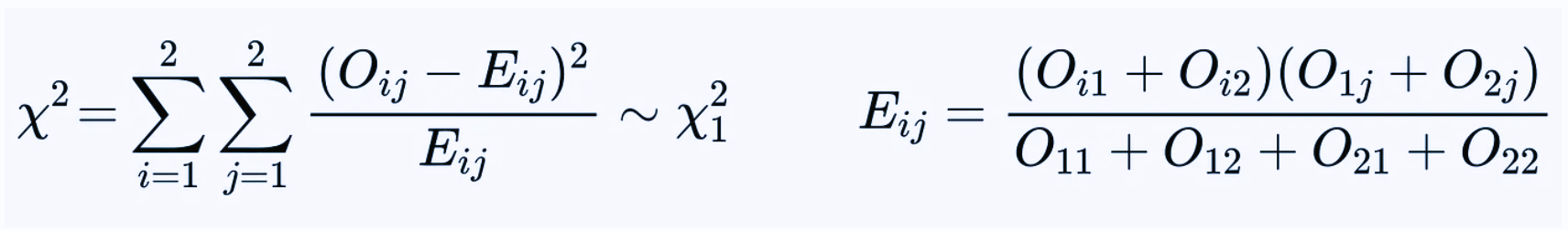
This test can also be used with non-normal observations if the sample size is large enough (central limit theorem).

In our example, using Pearson’s chi-square test we obtain χ2 ≈ 3.825, which gives p-value ≈ 5.1%.

Continuous metrics

Let’s now consider the case of a continuous metric such as the average revenue per user. We randomly show visitors one of two possible layouts of our website, and based on how much revenue each user generates in a month we want to determine if one of the two layouts is more efficient.

Let’s consider the following case.

• nX = 17 users saw the layout A, and then made the following purchases: 200$, 150$, 250$, 350$, 150$, 150$, 350$, 250$, 150$, 250$, 150$, 150$, 200$, 0$, 0$, 100$, 50$.
• nX = 14 users saw the layout B, and then made the following purchases: 300$, 150$, 150$, 400$, 250$, 250$, 150$, 200$, 250$, 150$, 300$, 200$, 250$, 200$.

Again, at a first glance, it looks like version B was more effective. But how statistically significant is this discrepancy?

Z-test

The Z-test can be applied under the following assumptions.

• The observations are normally distributed (or the sample size is large).
• The sampling distributions have known variance σX and σY.

Under the above assumptions, the Z-test exploits the fact that the following Z statistic has a standard normal distribution.

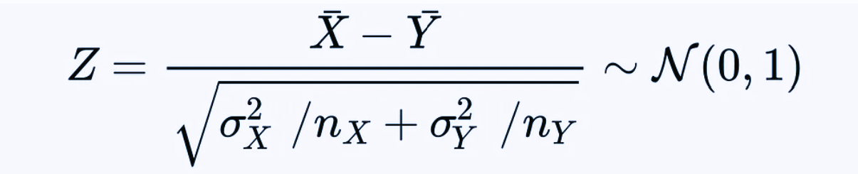
Unfortunately in most real applications the standard deviations are unknown and must be estimated, so a t-test is preferable, as we will see later. Anyway, if in our case we knew the true value of σX=100 and σX=90, then we would obtain z ≈ -1.697, which corresponds to a p-value ≈ 9%.

Student’s t-test

In most cases, the variances of the sampling distributions are unknown, so that we need to estimate them. Student’s t-test can then be applied under the following assumptions.

• The observations are normally distributed (or the sample size is large).
• The sampling distributions have “similar” variances σX ≈ σY.

Under the above assumptions, Student’s t-test relies on the observation that the following t statistic has a Student’s t distribution.

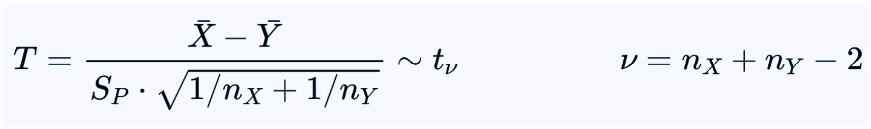
Here SP is the pooled standard deviation obtained from the sample variances SX and S Y, which are computed using the unbiased formula that applies Bessel’s correction.

In our example, using Student’s t-test we obtain t ≈ -1.789 and ν = 29, which give p-value ≈ 8.4%.

Welch’s t-test

In most cases Student’s t test can be effectively applied with good results. However, it may rarely happen that its second assumption (similar variance of the sampling distributions) is violated. In that case, we cannot compute a pooled variance and rather than Student’s t test we should use Welch’s t-test.

This test operates under the same assumptions of Student’s t-test but removes the requirement on the similar variances. Then, we can use a slightly different t statistic, which also has a Student’s t distribution, but with a different number of degrees of freedom ν.

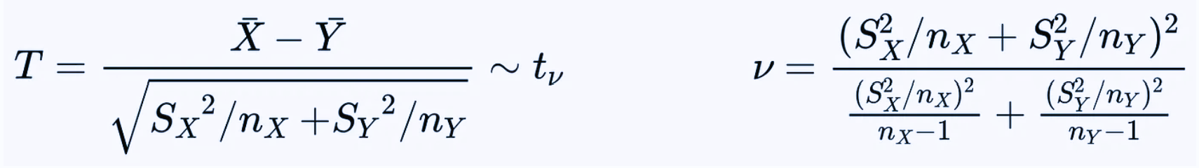
In our example, using Welch’s t-test we obtain t ≈ -1.848 and ν ≈ 28.51, which give p-value ≈ 7.5%.

Mann–Whitney U test This test makes no assumption on the nature of the sampling distributions, so it is fully nonparametric. The idea of Mann-Whitney U test is to compute the following U statistic.

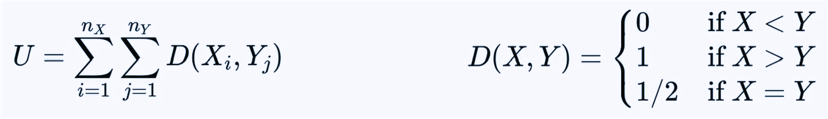
The values of this test statistic are tabulated, as the distribution can be computed under the null hypothesis that, for random samples X and Y from the two populations, the probability P(X < Y) is the same as P(X > Y).

In our example, using Mann-Whitney U test we obtain u = 76 which gives p-value ≈ 8.0%.

After seeing that different kinds of metrics, sample size, and sampling distributions require different kinds of statistical tests for computing the the significance of A/B tests. We can summarize it as:

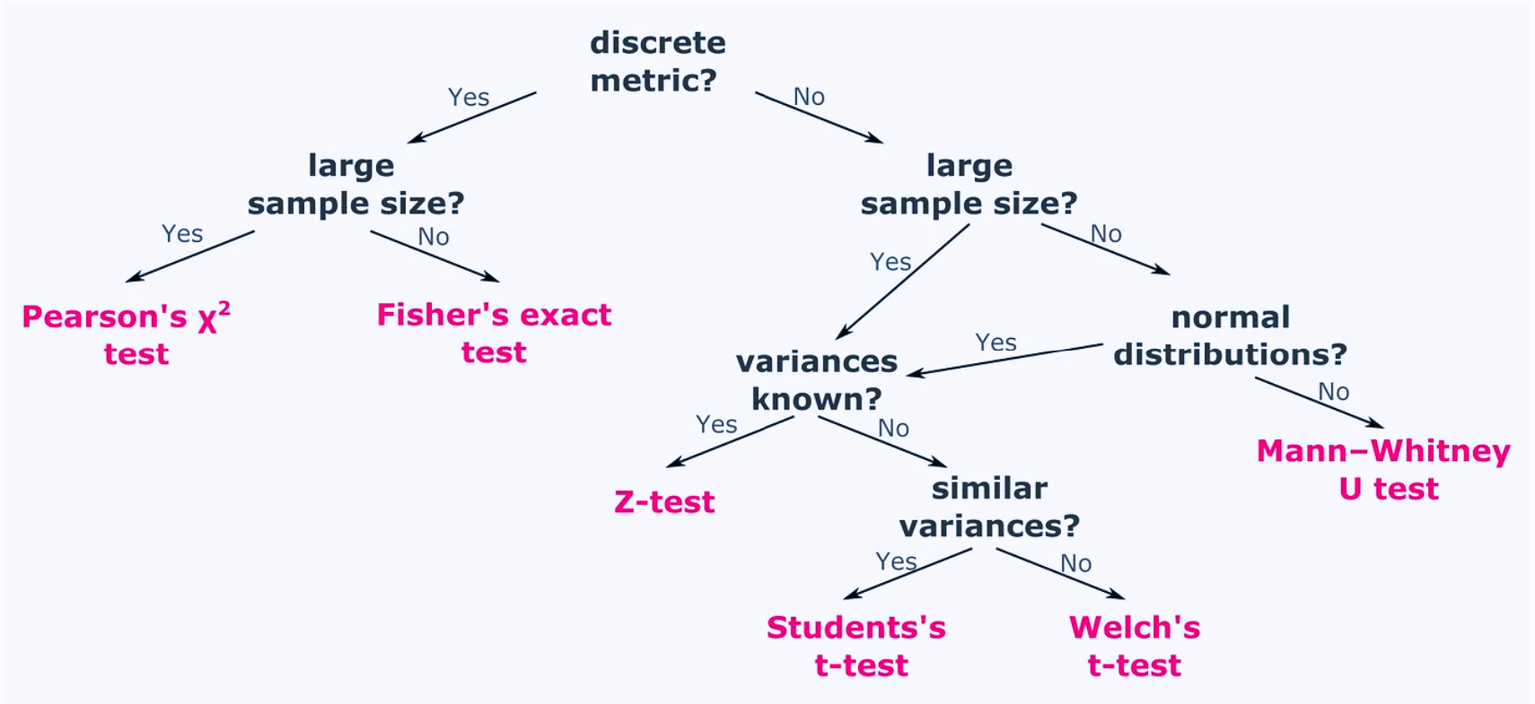
The code is available here.